Hanging chain 1

Fig.1. A hanging chain.

Fig.2. Simple suspension bridge.

 

Fig.3. Keleti Railway Station (Budapest, Hungary).

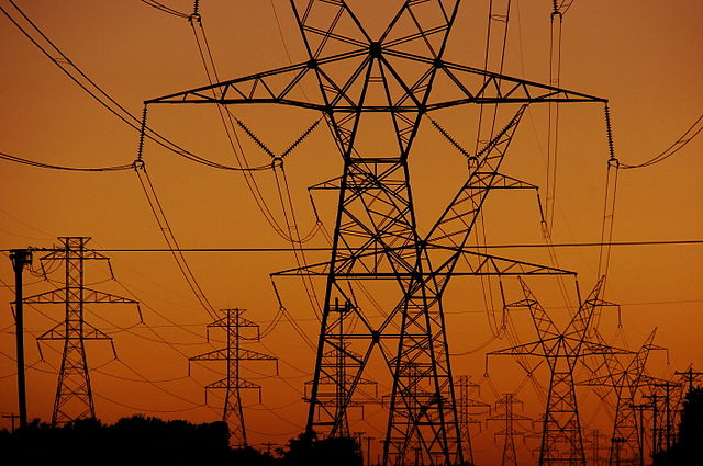
Fig.4. Freely-hanging electric power cables.

 

Problem 1.

Determine the shape of a hanging chain.

Show Solution

Let the chain be described by the function $y(x)$, and let the tension be described by the function $T(x)$. Consider a small piece of the chain, with endpoints at $x$ and $x + dx$, as shown below. Let the tension at $x$ pull downward at an angle $\theta_1$ with respect to the horizontal, and let the tension at $x + dx$ pull upward at an angle $\theta_2$ with respect to the horizontal. Balancing the horizontal and vertical forces on the small piece of chain gives $$\begin{align} T(x+dx)\cos(\theta_2)&=T(x)\cos(\theta_1),\nonumber \\ T(x+dx)\sin(\theta_2)&=T(x)\sin(\theta_1)+\frac{g\varrho dx}{\cos(\theta_1)},\label{eq:tension} \end{align}$$ where $\varrho$ is the mass per unit length. The second term on the right is the weight of the small piece, because $dx/ \cos(\theta_1)$ (or $dx/ \cos(\theta_2)$, which is essentially the same) is its length.
Squaring and adding eqs. $\eqref{eq:tension}$ gives $$\begin{equation*} [T(x+dx)]^2=[T(x)]^2+2T(x)g\varrho\tan(\theta_1)dx+O(dx^2). \end{equation*}$$ From this

$$\begin{align*} &\Step{1A}{[T(x+dx)-T(x)][T(x+dx)+T(x)]=2T(x)g\varrho\tan(\theta_1)dx+O(dx^2),}\\ &\Step{2A}{\frac{T(x+dx)-T(x)}{dx}[T(x+dx)+T(x)]=2T(x)g\varrho\tan(\theta_1)+O(dx),} \\ &\Step{3A}{\lim_{dx\to 0}\frac{T(x+dx)-T(x)}{dx}[T(x+dx)+T(x)]} \\ &\Step{4A}{\qquad\qquad\qquad\qquad\qquad\qquad\qquad=\lim_{dx\to 0}[2T(x)g\varrho\tan(\theta_1)+O(dx)],}\\ &\Step{5A}{\qquad T'(x)2T(x)=2T(x)g\varrho\tan(\theta_1),}\\ &\Step{6A}{\qquad T'(x)=g\varrho\tan(\theta_1).}\\ \end{align*}$$

Since $\tan(\theta_1)=y'(x)$, we obtain $$T'(x)=g\varrho y'(x).$$ Integrating both sides we get $$\begin{equation} \label{eq:T_and_y} T(x)=g\varrho y(x)+c_1, \end{equation}$$ where $c_1\in\mathbf{R}$ is an arbitrary constant.
Let’s see what we can extract from the first equation in eqs. $\eqref{eq:tension}$.
Using the trigonometrical identity $$\cos^2(z)=\frac{1}{1+\tan^2(z)}$$ it follows $$\cos^2(\theta_1)=\frac{1}{1+(y'(x))^2},$$ and $$\cos^2(\theta_2)=\frac{1}{1+(y'(x+dx))^2}.$$ Subtituting these into the first equation of $\eqref{eq:tension}$ we obtain $$\frac{T^2(x+dx)}{1+(y'(x+dx))^2}=\frac{T^2(x)}{1+(y'(x))^2},$$ or equivalently, $$\begin{equation} \label{eq:Ty} \frac{T^2(x+dx)}{T^2(x)}=\frac{1+(y'(x+dx))^2}{1+(y'(x))^2}. \end{equation}$$ Here $$\begin{align*} T^2(x+dx)&=[T(x)+T'(x)dx+O(dx^2)]^2\\ &=T^2(x)+2T(x)T'(x)dx+O(dx^2), \end{align*}$$ and assuming the existence of $y''(x)$ $$[y'(x+dx)]^2=[y'(x)]^2+2y'(x)y''(x)dx+O(dx^2).$$ Substituting these values into $\eqref{eq:Ty}$ we have $$2\frac{T'(x)}{T(x)}dx+O(dx^2)=2\frac{y'(x)y''(x)}{1+(y'(x))^2}dx+O(dx^2),$$ that is, $$\frac{T'(x)}{T(x)}-\frac{y'(x)y''(x)}{1+(y'(x))^2}=O(dx).$$ Taking $dx\to 0$ we obtain $$\frac{T'(x)}{T(x)}=\frac{y'(x)y''(x)}{1+(y'(x))^2}.$$ Integrating both sides gives $$\ln T(x)+c_2=\frac{1}{2}\ln(1+(y'(x))^2),$$ where $c_2\in\mathbf{R}$ is an arbitrary constant. Exponentiating gives $$\begin{equation} \label{eq:Typrime} c_3^2T^2(x)=1+(y'(x))^2, \end{equation}$$ where $c_3=e^{c_2}$.
We now consider eq. $\eqref{eq:Typrime}$ and $\eqref{eq:T_and_y}$. Eliminating $T(x)$ yields $c_3^2(g\varrho y(x)+c_1)^2=1+(y'(x))^2$. We can rewrite this in the somewhat nicer form, $$1+(y'(x))^2=\alpha^2(y(x)+h)^2,$$ where $\alpha=c_3g\varrho$, and $h=c_1/g\varrho$. We look for the non-constant solution. Separating the variables (it is enough to consider the $+$ sign) $$\frac{1}{\sqrt{\alpha^2 (y+h)^2-1}}dy=1 dx.$$ Integrating both sides (Hint: (a) $u:=\alpha (y+h)$ (b) $u:=\cosh(x)$ ) $$\frac{1}{\alpha}\ln\left(\alpha(h+y)+\sqrt{\alpha^2(h+y)^2-1}\right)=x+a,$$ where $a\in\mathbf{R}$ is an arbitrary constant.
From this $$\alpha(h+y(x))+\sqrt{\alpha^2(h+y(x))^2-1}=e^{\alpha(x+a)}.$$ Solving this equation for $h+y(x)$ we obtain $$\bbox[lightblue,5px,border:2px solid red]{\color{#800000}{ \bf{y(x)+h=\frac{1}{\alpha}\cosh[\alpha(x+a)].}}}$$